FYS4340/FYS9340 Diffraction methods and electron microscopy

Presentation on theme: "FYS4340/FYS9340 Diffraction methods and electron microscopy"— Presentation transcript:

1 FYS4340/FYS9340 Diffraction methods and electron microscopy
Autumn 2016

2

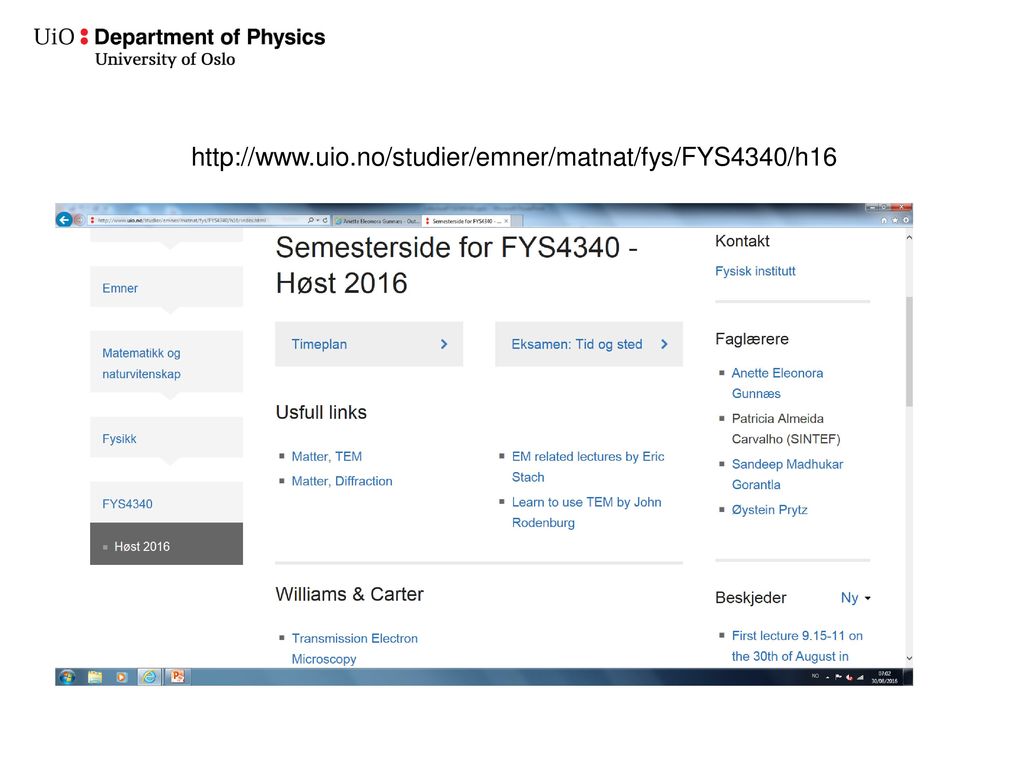
3 Preliminary teaching schedule
Lectures on Tuesdays 09:15-11:00 Exercises and lab on Thursdays 12:15-16:00 Not every Thursday, will be announced. Sometimes an extra lecture Nothing planned for this week or next

4 Contact info: Anette Gunnæs: Sandeep Gorantla: Patricia Carvalho: Øystein Prytz: TEM lab: Phuong D. Nguyen: Prep. lab: Ole Bjørn Karlsen: HMS officer: Cecilie Granerød:

5 Diffraction methods and electron microscopy
Williams & Carter. Transmission Electron Microscopy. 2nd ed. Springer, 2009. In particular parts 1,2, and 3 Various articles and papers (mandatory for PhD students) Additional suggested reading: Fultz and Howe: Transmission electron microscopy and diffractometry of materials. Both of these textbooks are available online on the UiO network.

6 Curriculum Instrumentation Specimen preparation Diffraction Imaging
Williams and Carter chapters: 1, 2, 3, 5, 6, 9 Specimen preparation Williams and Carter chapter: 10 Diffraction Williams and Carter chapters: 11, 12, 13, 16, 18, 19, 20, 21 Imaging Williams and Carter chapters: 22, 23, 24, 25, 26, 27, 28 EDS Williams and Carter chapters: not clarified yet

7 Why electron microscopy?
Many of the properties of a material are determined by its defects Precipitates and chemical segregation 2D defects: Interfaces and planar defects 1D defects: Dislocations 0D defects: Interstitials and substitutions Want to investigate these features on the relevant length scale

8 The first electron microscope
Knoll and Ruska, first TEM in 1931 Idea and first images published in 1932 By 1933 they had produced a TEM with two magnetic lenses which gave times magnification. Electron Microscope Deutsches Museum, 1933 model Ernst Ruska: Nobel Prize in physics 1986

9 The first commercial microscopes
1939 Elmiskop by Siemens Company 1941 microscope by Radio corporation of America (RCA) First instrument with stigmators to correct for astigmatism. Resolution limit below 10 Å. Elmiskop I

10 Observations of dislocations and lattice images
1956 independent observations of dislocations by: Hirsch, Horne and Wheland and Bollmann -Started the use of TEM in metallurgy. 1956 Menter observed lattice images from materials with large lattice spacings. 1965 Komoda demonstrated lattice resolution of 0.18 nm. One exceptions was the work of yada who got crystallographic information from chrysotile fibres

11 Menter,

12 Use of high resolution electron microscopy (HREM) in crystallography
1971/72 Cowley and Iijima Observation of two-dimensional lattice images of complex oxides 1971 Hashimoto, Kumao, Hino, Yotsumoto and Ono Observation of heavy single atoms, Th-atoms Th-compound supported on a graphite thin crystal film. Bright spots attributed to single Th atoms.

13 1970’s Early 1970’s: Development of energy dispersive x-ray (EDX) analyzers started the field of analytical EM. Development of dedicated HREM Electron energy loss spectrometers and scanning transmission attachments were attached on analytical TEMs. Small probes making convergent beam electron diffraction (CBED) possible.

14 1980’s and 90’s Development of combined high resolution and analytical microscopes. An important feature in the development was the use of increased acceleration voltage of the microscopes. Field Emission Guns (FEG) Development of Cs and Cc correction Probe and image Improved energy spread of electron beam More user friendly Cold FEG Monocromator 2000’s

15 Eric Stach (2008), ”MSE 528 Lecture 4: The instrument, Part 1, http://nanohub.org/resources/3907

16 Apertures

17 The effect of accelerating the electron
U k = λ-1 (nm-1) λ (nm) m/mo v/c 1 V 0.815 1.226 0.0020 10 V 2.579 0.3878 0.0063 100 V 8.154 0.1226 0.0198 10 kV 81.94 0.1950 100 kV 270.2 1.1957 0.5482 200 kV 398.7 1.3914 0.6953 10 MV 8468 0.9988 Relations between acceleration voltage, wavevector, wavelength, mass and velocity

18 The requirements of the illumination system
High electron intensity Image visible at high magnifications Small energy spread Reduce chromatic aberrations effect in obj. lens Adequate working space between the illumination system and the specimen High brightness of the electron beam Reduce spherical aberration effects in the obj. lens Has to produce a uniform distribution of electrons on the specimen. Chromatic aberration skisse Spherical aberration skisse Why do we want working space?

19 The electron source Two types of emission sources Thermionic emission
LaB6 Field emission ZrO/W Cold FEG Schottky FEG

20 Thermionic guns Filament heated to give Thermionic emission
Tungsten (W) Lanthanum hexaboride (LaB6) Filament negative potential to ground Wehnelt produces a small negative bias Brings electrons to cross over

21 The Field emission gun (FEG)
The principle: The strength of an electric field E is considerably increased at sharp points. E=V/r rW < 0.1 µm, V=1 kV → E = 1010 V/m Lowers the work-function barrier so that electrons can tunnel out of the tungsten. Three main parts and acts as an acceleration triode. These parameters are interrelated and can be varied to optimize the performance of the gun. Limited by the the properties of the electron source.

22 Electron lenses Electrostatic Electromagnetic F= -eE F= -e(v x B)
Any axially symmetrical electric or magnetic field has the properties of an ideal lens for paraxial rays of charged particles. Electrostatic Require high voltage - insulation problems Not used as imaging lenses, but are used in modern monochromators or deflectors Electromagnetic Can be made more accurately Shorter focal length F= -eE F= -e(v x B) Paraxial rays: rays close to the optcal axis. Wien filter

23 Electromagnetic lens Current in the coil creates
Bore Current in the coil creates A magnetic field in the bore. The magnetic field has axial symmetry, but is inhomogenious along the length of the lens. Soft Fe pole piece gap Cu coil The soft iron core can increase the field by several thousand times.

24 General features of electromagnetic lenses
Focuses near-axis electron rays with the same accuracy as a glass lens focuses near axis light rays. Same aberrations as glass lenses. Converging lenses. The bore of the pole pieces in an objective lens is about 4 mm or less. A single magnetic lens rotates the image relative to the object. Focal length can be varied by changing the field between the pole pieces (changing magnification).